Developed by Jordan Mecom, Alice Wang, and Will Hardy.
View the repository here.
Motivation and Problem Defintion
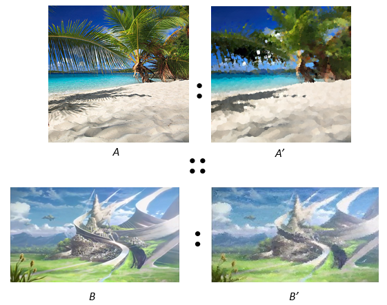
Image Analogies, by Hertzmann et. al develops a framework which can create new images from a single training example. This is done through the idea of an image analogy: take an image A and its transformation A’, and provide any image B to produce an output B’ that is analogous to A’. Or, more succinctly: A : A’ :: B : B’. Hertzmann’s algorithm attempts to learn complex, non-linear transformations between A and A’, allowing them to be applied to any other image. This provides a much more powerful and intuitive model than manually selecting filters from a list.
More formally, the inputs and ouputs are
Input: Three images - unfiltered A, filtered A’, and unfiltered target B. A and A’ must be registered: “the colors at and around any pixel in A correspond to the colors at and around the same pixel in A’”.
Output: Filtered target image B’ such that A : A’ :: B : B’.
Related Work
Our implementation of image analogies replicates the psuedocode described in the original Image Analogies paper. This algorithm is similar in nature to image quilting, which we previously implemented. The fundamental idea of synthesizing a new image one pixel at a time, by finding a best matching pixel through some statistical measure, is drawn from related work on texture synthesis and is core to the image analogies algorithm.
Algorithm
The general idea of image analogies is to, for each layer in a Gaussian pyramid, iterate over each pixel, q, in B’, and find some pixel, p from A’ that is the best match to q. The relevant features from p are then copied over into B’, and the finest B’ layer from the pyramid is then returned. Our implementation is described more precisely in the pseudocode below:
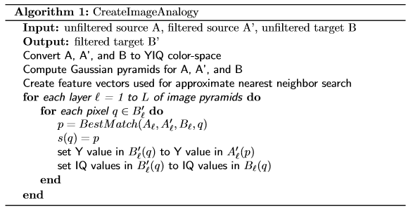
We convert to YIQ color space because the the only feature that we use to compute best matches is luminance. The paper notes that, in special cases, other features such as steerable filters may be used, but almost every application of image analogies only uses luminance. Gaussian pyramids are computed so that the BestMatch algorithm is more accurate. The feature vectors for the nearest neighbor search are, for each pixel, a 5 by 5 neighborhood of the luminance values around and of that pixel.
The main loop iterates over each layer of the image pyramid, and then calculates the best matching pixel for the current pixel in B’ using the BestMatch routine. Once the optimal pixel is found, the map s(q) = p is updated. This map simply records the mapping from q in B’ to p in A’, as it makes parts of BestMatch more efficient. The luminance value in B’ is then set to the luminance value in A(p) at the current layer, l. Then the color of B’ is restored by copying the color from B at the current pixel being synthesized, q, over to B’.
The BestMatch routine, and its subroutines, are described below:
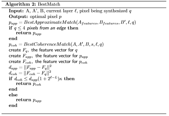
BestMatch returns the pixel from BestApproximateMatch or BestCoherenceMatch. The approximate-match pixel is the one returned from an approximate nearest neighbor search. This approximate-match pixel is essentially guaranteed to have the closest luminance to the pixel being synthesized. However, this is not always perceptually optimal because it’s not necessarily coherent with the pixels already synthesized in B’. Thus, BestMatch compares the results from BestApproximateMatch and BestCoherenceMatch using a distance function and then returns the best result.
The edge case checked at the top - if q is near a border - simplifies any edge cases regarding odd neighborhood sizes in best coherence match. The paper says to use “brute force” in these cases, so the result should be similar.
The feature vectors F(.) are used to calculate which pixel to return. So, F(q) is the concatenation of a 5*5 neighborhood around q in B(l) and B’(l), and a 3x3 neighborhood around B(l-1) and B’(l-1). Note that, we do not include non-synthesized pixels in F. Hence the pixels that come from the fine layers don’t use the complete 5x5 neighborhood. Typically, instead, they are in L shape. However, the full neighborhoods from the coarse layers are always used. Also note that in this notation, F(.) is the feature vector around a pixel in either the (A, A’) pairs or the (B, B’) pairs.
Once the feature vectors are computed, the pixels must be compared using some distance metric. We use an L2-norm, however we preprocess F such that each neighborhood being concatenated is weighted using Gaussian weights centered around the argument pixel, and is also normalized so that the fine and coarse layers are equally weighted.
Now, once we have the distances for the approximate and coherence pixels, we compare which to use. Since the approximate pixel will almost always be better, it’s artifically weighted. The paper notes that this weighting scheme is essentially estimating the scale of the “textons” at level l. After this weight, the optimal pixel is returned.
The algorithm for BestApproximateMatch simply returns the result from an approximate nearest neighbor search using feature vectors from A’ using a query feature vector from the current pixel being sythesized. To implement this, we used an ANN library found here.
BestCoherenceMatch returns s(r*) + (q - r*), where r* is defined as
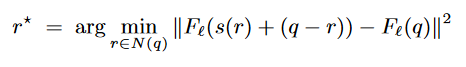
N(q) is the neighborhood of already synthesized pixels adjacent to q in B’. As noted above, the aim is to return a pixel that is coherent with the neighborhood around the already synthesized portion of B’. This allows for the texture of some filters (such as oil paintings) to come through.
Results
Sanity check
We first tested with no filter (the paper refers to this as identity filter), setting kappa = 0, to confirm that the algorithm works.
| A | A’ |
|---|---|
 |
|
| B | B’ |
 |
 |
While not perfectly reconstructing the original image (there’s very slight blurring), our result is as good as the result from the paper.
Filters
From there, we tried some simple filters. The first is brightness, with kappa = 0.5.
| A | A’ |
|---|---|
 |
 |
| B | B’ |
 |
 |
This result worked quite well. This is expected, since the filter is essentially just the identity test plus a scalar luminance factor.
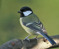
Next we tried a contrast filter, with kappa = 0.5.
| A | A’ |
|---|---|
 |
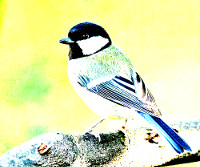 |
| B | B’ |
 |
 |
Contrast also performed well, for the most part. However, it had some black artificats. There is some strange behavior even in the original A’ filter though – notice the bright green spot to the left of the bird.
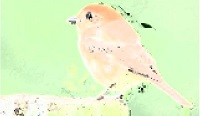
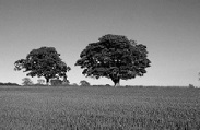
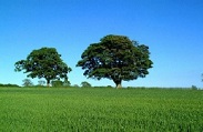
Recolorization
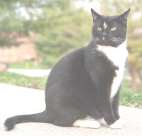
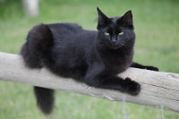
We tried the recolorization example in the paper. In each recolorization case, kappa = 2:
| A | A’ |
|---|---|
 |
 |
| B | B’ |
 |
 |
Our result is basically identical to the example in the paper, found here. However, recolorization doesn’t always work so well. Perhaps this is why they only show off one example.
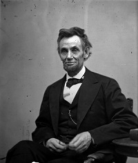
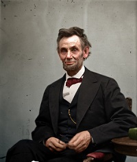
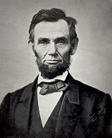
Here’s our attempt with Abe Lincoln.
| A | A’ |
|---|---|
 |
 |
| B | B’ |
 |
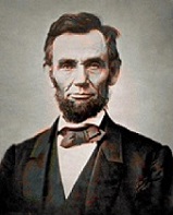 |
While there was some attempt at recoloring his jacket, the algorithm basically failed here. The examples that paper shows essentially are monotone and only have a few colors that cover large portions of the image with strong edges between regions. If the range of colors in the images to be recolorized is narrow, then we expect the filter to be less successful and often remap, say, grey to beige for example.
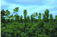
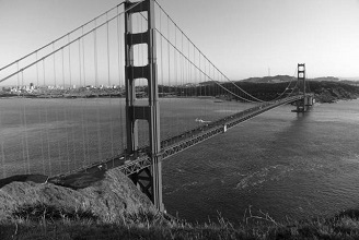
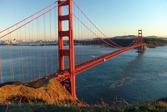
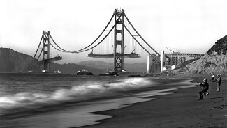
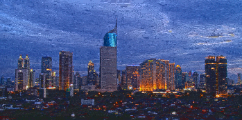
And one more attempt at recolorization: we tried to colorize a photo of the Golden Gate Bridge in construction using a current photo of the bridge.
| A | A’ |
|---|---|
 |
 |
| B | B’ |
 |
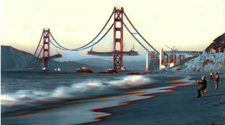 |
The bridge is recolored pretty well, because it has strong edges and a drastic color shift. However, the landscape - most notably the sand - has lots of small gradients, which this method has a difficult time finding good matches for.
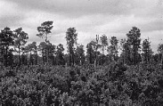
Artistic filters
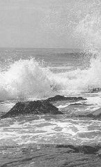
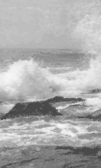
The rest of our results consist of artistic filters. We first attempted the Rhone data from the paper, using kappa = 0.5.
| A | A’ |
|---|---|
 |
 |
| B | B’ |
 |
 |
This result was pretty good, but didn’t quite capture the original scale of the texture from the Rhone image. One reason for this is that we have to scale all of our images down to run our algorithm, because the running time for our implementation is incredibly slow (discussed further below). This means that the texture is lost as the image is scaled down. Another reason is that kappa = 0.5, whereas the paper suggests a range of 2 to 25. We would have tested on more ranges, but we didn’t have time (see below).
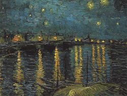
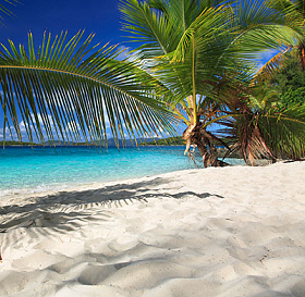
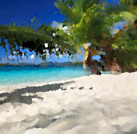
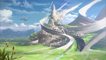
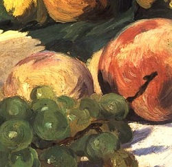
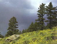
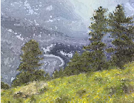
Next we tested using some original data, with kappa = 2.
| A | A’ |
|---|---|
 |
 |
| B | B’ |
 |
 |
We were quite pleased with this result, especially given our inability to parameter tune. The oil painting texture is reproduced very well.
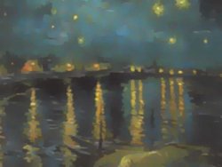
Actually, we liked the oil painting so much, we did some more. Kappa = 2 here as well.
| A | A’ |
|---|---|
|
|
| B | B’ |
 |
 |
Pretty! Here, the original input was already a painting. We simply transfered a different style over to it.
We were unable to reproduce one example from the paper. Here we used kappa = 5.
| A | A’ |
|---|---|
 |
 |
| B | B’ |
 |
 |
The output here is pretty bad. While it does capture some of the texturing, there is severe noise and white patches. This is the only test data from the paper that we couldn’t reproduce. We suspect that this is because our luminance remapping does not work correctly. The paper highlighted the importance of luminance remapping in only the artistic style transfer case, and since this is the only case we couldn’t reproduce the paper’s results, we think this must be why.
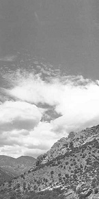
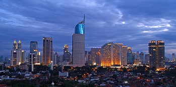
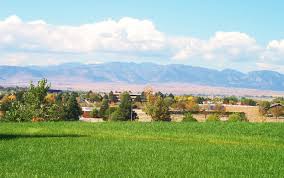
And last, another failure case with original data. We set kappa = 10 here.
| A | A’ |
|---|---|
|
|
| B | B’ |
 |
 |
This is probably our worst result. Again, this may be attributed to luminance remapping. Another idea is that the blurry input from Rhone (in A) lacks any strong edges. However, there are many strong edges in B which may disrupt the texture. Still, that doesn’t quite explain the problems in the sky. Ultimately, we aren’t quite sure why this one failed so drastically. Perhaps tuning parameters, such as kappa or the number of layers in the image pyramid, could yield better results.
Analysis
The image analogies framework is overall quite impressive. It does a good job of reproducing the effects of filtering techniques that would be nearly impossible to characterize mathematically. The paper gives some examples where it succeeds greatly, and we were able to find some original cases that also looked very good. However, the algorithm is still very sensitive to input data and parameters, which may require a good deal of tuning to use effectively. This limits its practical use cases. Most importantly, it can be very difficult to pick inputs that will yield positive results.
Furthermore, the algorithm is incredibly slow. It must perform a k-nearest-neighbor search for each pixel, assuming 5x5 neighborhoods and image size w*h, on a matrix of size 25 * (w*h). This can be very unweildy. The coherence match isn’t as computationally expensive, but still must pick out the best pixel in a neighborhood of at most size 13 for each pixel, which themselves are matched to an additional neighborhood. And of course, it must do all this for multiple layers of an image pyramid.
The primary challenge we faced was dealing with speed. We believe our main problem is tied to our choice of MATLAB. We’re aware of other implementations (such as the original paper) in C++ that perform much better. For example, even if we only use ANN search using a MATLAB wrapper around a C++ library, we still have runtimes 30 - 60x worse on images that were less half the size. We profiled our code using MATLAB’s code profiler, and were able to optimize the code that we had written (outside of the ANN library), increasing efficiency by 50%. Still, we weren’t able to overcome multiple-hour long runtimes, making it very hard to tune parameters.